Trees are one of the ways to represent hierarchical structures and thus are used in many problem domains. This article discusses the four most popular ways of representing trees in RDBMS by using an example from a simple problem domain.
Representing and storing data in a tree-like structure is a common problem in software development:
- XML/Markup syntax parsers, such as Apache Xerces and Xalan XSLt, use trees;
- PDF uses the following tree structure: root node -> catalog node -> page nodes -> child page nodes. Usually PDF files are represented in memory as balanced trees;
- multiple scientific and gaming applications employ decision trees, probability trees, behavioral trees; the Flare visualization library (http://flare.prefuse.org/) makes ample use of spanning trees, trees are also used by brokers when they decide whether to tender for a contract.
Trees are one of the ways to represent hierarchical structures and thus are used in many problem domains:
- binary tree in computer science,
- phylogenetic tree in biology,
- Ponzi scheme in business,
- task decomposition tree in project management,
- trees are used to model multilevel relationships, such as “superior - subordinate”, “ancestor - descendant”, “whole - part”, “general - specific”.
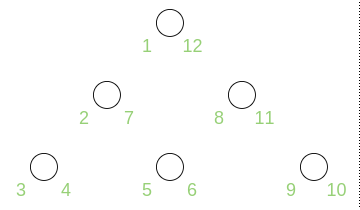
This article discusses the four most popular ways of storing trees in a relational database. As an example we will use a catalog of construction supplies (fig. 1) and the Postgres 9.6 RDBMS.
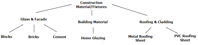
Fig. 1. Construction supplies catalog
Graph theory uses the term “tree” to denote acyclic connected graphs, while the term “forest” is used for arbitrary acyclic graphs (possibly disconnected). The methods discussed in this article can be applied both for storing trees and forests without loss of generality.
1. Adjacency list
Adjacency lists in graph theory is a way to represent a graph by storing a list of neighbors (that is, adjacent vertices) for each vertex. For trees it is possible to store only the parent node, and then each of these lists contains a single value that can be stored in a database along with the vertex. This is one of the most popular representations, and also the most intuitive one: the table only has references to itself (fig. 2). Root node then contains an empty value (NULL) for their parent.
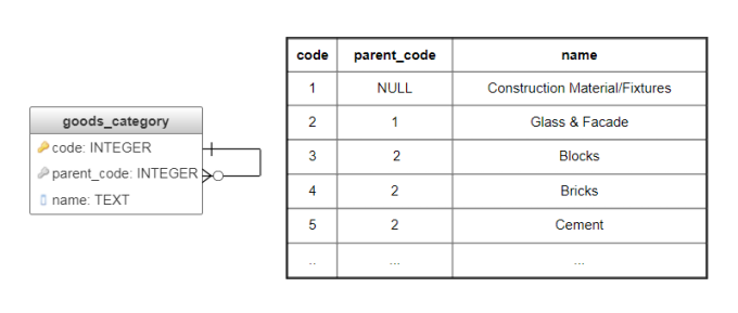
Fig. 2. Adjacency list implementation
Main data selection operations for this method require DBMS to support recursive queries. PostgreSQL supports this type of queries, but with DBMS that doesn’t you might need to perform the selection by employing temporary tables and stored procedures. Following are some query examples.
Getting the subtree for the given node:
WITH RECURSIVE sub_category(code, name, parent_code, level) AS (
	SELECT code, name, parent_code, 1 FROM goods_category WHERE code=1 /* id of the given node */
	UNION ALL
	SELECT c.code, c.name, c.parent_code, level+1
	FROM goods_category c, sub_category sc
	WHERE c.parent_code = sc.code
)
SELECT code, name, parent_code, level FROM sub_category;
Path to the given node from the root:
WITH RECURSIVE sub_category(code, name, parent_code, level) AS (
	SELECT code, name, parent_code, 1 FROM goods_category WHERE code=5 /* id of the given node */
	UNION ALL
	SELECT c.code, c.name, c.parent_code, level+1
	FROM goods_category c, sub_category sc
	WHERE c.code = sc.parent_code
)
SELECT code, name, parent_code, (SELECT max(level) FROM sub_category) - level AS distance FROM sub_category;
Check if the Cement node (code = 5) is a descendant of Construction Material/Fixtures(code=1):
WITH RECURSIVE sub_category(code, name, parent_code, level) AS (
	SELECT code, name, parent_code, 1 FROM goods_category WHERE code=5 /* id of the checked node */
	UNION ALL
	SELECT c.code, c.name, c.parent_code, level+1
	FROM goods_category c, sub_category sc
	WHERE c.code = sc.parent_code
)
SELECT CASE WHEN exists(SELECT 1 FROM sub_category WHERE code=2 /* code of the subtree root */)
	THEN 'true'
	ELSE 'false'
	END
Advantages of this method include:
- intuitive representation of the data (tuples
(code, parent_code)directly correspond to the tree edges); - there is no data redundancy, and there is no need for non-referential integrity constraints (unless you need DBMS-level constraints for preventing cycles);
- trees can have arbitrary depth;
- fast and simple insert, move, and delete operations, since they don’t affect any additional nodes.
The disadvantage is that:
- the method requires recursion in order to select node’s descendants or ancestors, to define the depth of the node, and to find out the number of descendants; if the DBMS doesn’t support specific features, these operations can’t be implemented efficiently. For the situations when recursion is either not possible or not feasible, some of the advantages of this method can be achieved by employing a flat table.
2. Subsets
Also known as Closure table or Bridge table.
This method represents trees as nested subsets: the root node contains all nodes with depth level 1, they in turn contain nodes with depth level 2 and so on (fig. 3).
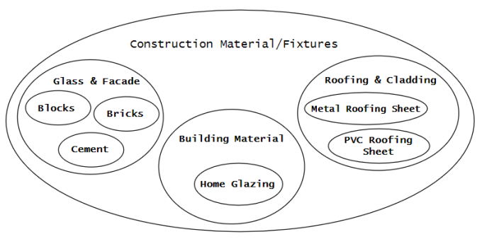
Fig 3. Representing trees as nested subsets
The Subsets method requires two tables: the first table contains all subsets (table goods_category, fig. 4), the second contains facts of inclusion for the subsets, along with the corresponding level of depth (table subset, fig. 4).
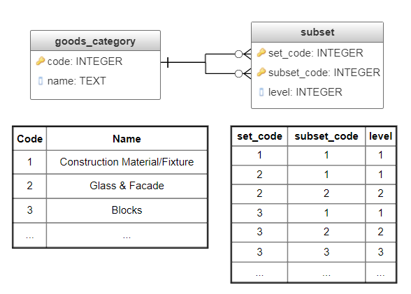
Fig. 4. Subsets implementation
As a result, for each node in the tree, the subset table contains number of records equal to the node’s depth level. Consequently, the number of records grows in arithmetic progression, however common queries become simpler and faster than in the previous method.
Getting the subtree for the given node:
SELECT name, set_code, subset_code, level FROM subset s
    LEFT JOIN goods_category c ON c.code = s.set_code
WHERE subset_code = 1 /* the subtree root */
ORDER BY level;
Path to the given node from the root:
SELECT name, set_code, subset_code, level FROM subset s
    LEFT JOIN goods_category c ON c.code = s.subset_code
WHERE set_code = 3 /* the give node */
ORDER BY level;
Check if the Blocks node (code = 3) is a descendant of Construction Material/Fixtures(code=1):
SELECT CASE
    WHEN exists(SELECT 1 FROM subset
                WHERE set_code = 3 AND subset_code = 1)
	THEN 'true'
	ELSE 'false'
	END
In order to preserve integrity, the move and insert operations require implementing triggers, that would update all associated records.
The main advantage of the Subsets method is support for fast, simple, non-recursive tree operations: subtree selection, ancestors selection, calculation of the node’s depth level and number of descendants.
Disadvantages include:
- relatively unintuitive data representation (it is complicated by redundant references between indirect descendants);
- data redundancy;
- triggers are required for data integrity;
- the move and insert operations are more complicated than for the Adjacency list method. Insertion requires additional records for every descendant node, while moving the node requires updating records for both its descendants and ancestors.
3. Nested sets
The idea of this method is to store the prefix traversal of the tree. Here the tree root is visited first, then all the nodes of the left subtree are visited in the prefix order, then the nodes of the right subtree are visited once again in the prefix order. The order of traversal is stored in two additional fields: left_key and right_key. The left_key field contains the number of traversal steps before entering the subtree, while the right_key contains the number of steps before leaving the subtree. As a result, for each node its descendants have their numbers between the node’s numbers, independently of their depth level. This property allows writing queries without employing recursion.
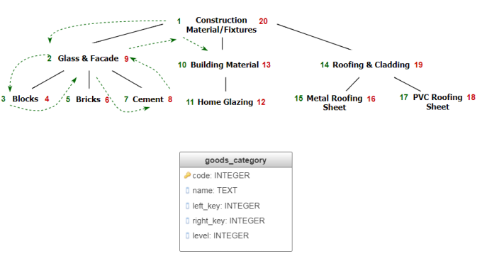
Fig. 5 Nested sets implementation
Getting the subtree for the given node:
WITH root AS (SELECT left_key, right_key FROM goods_category WHERE code=2 /* id of the node */)
SELECT * FROM goods_category
    WHERE left_key >= (SELECT left_key FROM root)
        AND right_key <= (SELECT right_key FROM root)
ORDER BY level;
Path to the given node from the root:
WITH node AS (SELECT left_key, right_key FROM goods_category WHERE code=8 /* id of the node */)
SELECT * FROM goods_category
    WHERE left_key <= (SELECT left_key FROM node)
        AND right_key >= (SELECT right_key FROM node)
ORDER BY level;
Check if the Blocks node is a descendant of the Construction Material/Fixtures node :
SELECT CASE
    WHEN exists(SELECT 1 from goods_category AS gc1, goods_category gc2
        WHERE gc1.code = 1
            AND gc2.code = 3
            AND gc1.left_key <= gc2.left_key
            AND gc1.right_key >= gc2.right_key)
    THEN 'true'
    ELSE 'false'
END
Benefit of this method is that it allows fast and simple operations for selecting the node’s ancestors, descendants, their count and depth level, all without recursion.
The main downside of the method is the necessity to reassign the traversal order when inserting or moving a node. For example, in order to add a node to the bottom level, it is necessary to update the left_key and right_key fields for all nodes to its “right and above”, which might require re-traversing the whole tree. It is possible to reduce the number of updates by assigning left_key and right_key values with an interval, e.g. 10 000 and 200 000 instead of 1 and 20. This will allow inserting a node without renumbering the others. Another approach would be to use real numbers for values of left_key and right_key.
4. Materialized paths
Also known as Lineage column
The idea of this method is to explicitly store the whole path from the root as a primary key for the node (fig. 6). Materialized paths is an elegant way of representing trees: every node has an intuitive identifier, individual parts of which have well-defined semantics. This property is very important for general-use classifications, including International Classification of Diseases (ICD), Universal Decimal Classification (UDC), used in scientific articles, PACS (Physics and Astronomy Classification Scheme). Queries for this method are concise, but not always efficient, since they involve substring matching.
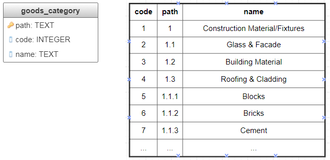
Fig. 6 Materialized paths implementation
Getting the subtree for the given node:
SELECT * FROM goods_category WHERE path LIKE '1.1%' ORDER BY path
Path to the given node from the root:
SELECT * FROM goods_category WHERE '1.1.3' LIKE path||'%' ORDER BY path
Check if the Cement node is a descendant of the Construction Material/Fixtures node:
SELECT CASE
    WHEN exists(SELECT 1 FROM goods_category AS gc1, goods_category AS gc2
        WHERE gc1.name = 'Construction Material/Fixtures'
            AND gc2.name = 'Cement'
            AND gc2.path LIKE gc1.path||'%')
    THEN 'true'
    ELSE 'false'
END
For cases when the number of levels and the number of nodes at each level is known in advance, it is possible to avoid using explicit separators by using numerical identifiers with strictly defined zero-padded groups of decimal places. This approach is used in many classifications, including OKATO, NAICS.
It is also possible to use separate columns for individual levels of hierarchy (multiple lineage columns): this will eliminate necessity to use substring matching.
Advantages of the Materialized paths method are intuitive representation of the data, as well as simplicity of some common queries.
Disadvantages of the method include complicated insert, move, and delete operations, non-trivial implementation of integrity constraints, as well as inefficient queries due to necessity to do substring matching. Another possible disadvantage is limited number of depth levels in case the numerical identifiers approach is used.
4.1. Ltree module for PostgreSQL
PostgreSQL has a designated ltree module for working with trees: it allows employing efficient implementation of the Materialized paths method in a convenient manner. The module implements an ltree data type for representing labels of data stored in a hierarchical tree-like structure. Extensive facilities for searching through label trees are provided.
Labels consist of alpha-numeric characters and underscores, and each label should be less than 256 bytes long (e.g. L1, 42, building_materials).
Path from the root to a particular node is stored as a dot-separated sequence of labels (e.g. L1.L2.L3), with maximum possible length equal to 65 Kb, though paths less than 2 Kb are preferable. The documentation states that this is not a major limitation, providing an example of DMOZ directory (http://dmoztools.net/) that has its largest label path only about 240 bytes long.
The module supports two types of templates for performing search on labels: lquery (regular expression for matching ltree values) and ltxtquery (fulltext ltree search template). The key difference between the two is that ltxtquery matches words independently of their position in the label path.
Let’s see how to perform common operations on our example tree with ltree.
First, we set up the module, create the table and fill it with data.
CREATE EXTENSION "ltree";

CREATE TABLE goods_category_ltree (path ltree, name text);

INSERT INTO goods_category_ltree (path, name) VALUES
    ('construction_materials', 'Construction Material/Fixtures'),
    ('construction_materials.glass', 'Glass & Facade'),
    ('construction_materials.building_materials', 'Building Material'),
    ('construction_materials.roofing', 'Roofing & Cladding'),
    ('construction_materials.glass.blocks', 'Blocks'),
    ('construction_materials.glass.bricks', 'Bricks'),
    ('construction_materials.glass.cement', 'Cement'),
    ('construction_materials.building_materials.home_glazing', 'Home Glazing'),
    ('construction_materials.roofing.metal_sheet', 'Metal Roofing Sheet'),
    ('construction_materials.roofing.pvc_sheet', 'PVC Roofing Sheet');
Getting the subtree for the given node:
SELECT * FROM goods_category_ltree WHERE path @> (SELECT path FROM goods_category_ltree WHERE name = 'Blocks');
or
SELECT path, name FROM goods_category_ltree WHERE path ~ 'construction_materials.glass.*';
Path to the given node from the root:
SELECT * FROM goods_category_ltree WHERE path <@ (SELECT path FROM goods_category_ltree WHERE name = 'Construction Material/Fixtures');
Check if the Cement node is a descendant of the Construction Material/Fixtures node:
SELECT CASE WHEN exists(SELECT 1 FROM goods_category_ltree
    WHERE (
        SELECT path FROM goods_category_ltree WHERE name = 'Construction material/ Fixtures'
    ) @> (SELECT path FROM goods_category_ltree WHERE name = 'Cement'))
THEN 'true'
ELSE 'false'
END
Determine the number of labels in a path (the depth level):
SELECT path, nlevel(path) FROM goods_category_ltree WHERE name ='Blocks';
Conclusion
We’ve discussed four most popular methods for storing tree-like structures in relational databases. Every method has its benefits and drawbacks.
Out of the four, only the Adjacency list method avoids redundancy and doesn’t require non-referential integrity constraints; insert and move operations don’t affect other records in the database. However, at least some kind of recursion is necessary for most queries.
The three other methods don’t need recursion for their queries, however insert and move operations can’t be performed without updating other associated nodes. The materialized paths and nested sets methods have possible optimizations, which deal only with some of their limitations.
The following figures use green color to schematically denote what data is actually stored in relational database for each of the discussed tree storage methods.
| Adjacency list | Subsets |
|---|---|
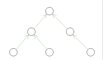 |
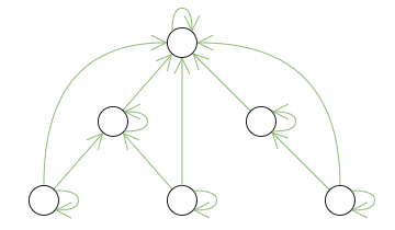 |
| Nested sets | Materialized paths |
|---|---|
 |
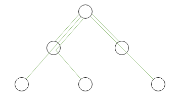 |
For the Adjacency list and Materialized paths methods, the stored data directly reflects initial structure of the domain. For the Subsets method the structure is complicated by additional reflexive and transitive connections between ancestors and descendants. The stored data of the Nested sets method is only indirectly relevant to the initial structure.
| Adjacency list | Subsets | Nested sets | Materialized paths | |
|---|---|---|---|---|
| Correlation of tree depth and subtree search time | significant: every new level of depth adds another recursive SELECT |
moderate | moderate, it is possible to create indices for left_key and right_key |
significant (substring matching). Employment of the ltree module might speed up the operations, since it supports several index types (B-tree and GiST over ltree values) |
| Node insertion | simple: doesn’t affect other records | complex: the node needs to be added to two tables, + new records for every descendant node | complex: requires updating all nodes “to the right and above” | complex: requires updating all descendant nodes |
| Node moving | simple: doesn’t affect other records | complex: requires updating records for the node’s ancestors and descendants | complex: requires updating all nodes “to the right and above” | complex: requires updating descendant and ancestor nodes |
| Node deletion | Simple, cascade | simple, cascade | simple | complex, substring matching |
| Redundancy | no | yes | yes | yes |
| Non-referential integrity constraints | not needed | needed | needed | needed |